
A practical guide to getting started in Deep Learning
Note: This article was originally published in Towards Data Science on December 30, 2020.
What is Deep Learning?
Deep learning is a subset of machine learning algorithms that use neural networks to learn complex patterns from large amounts of data.
Due to advances in computing and the amount of data being acquired, these algorithms are being applied in a wide range of problems ranging from self-driving cars to automated cancer detection.
What are Common Libraries for Deep Learning?
Several programming languages have developed software packages for deep neural network model development, such as TensorFlow and Pytorch.
While these open-source frameworks facilitate deep learning development, there is a bit of a learning curve to applying these frameworks for training neural networks.

Why use MATLAB for Deep Learning?
The Deep Learning Toolbox (DLT) is another tool that allows for quick prototyping and experimenting with neural network architectures.
Additionally, DLT hides many low-level details that go into designing a neural network, making it easy for beginners to understand the high-level concepts.
In this three-part series of articles, I will demonstrate some of the useful features of the DLT and apply the toolbox to address different problems we face in Deep Learning.
This first article will train a shallow neural network on the data to predict cancer malignancy using the Breast Cancer Wisconsin (Diagnostic) Data Set built into MATLAB.
The Breast Cancer Wisconsin (Diagnostic) Data Set
First, I’ll briefly describe the dataset, which was obtained from 699 biopsies. Each feature in the cancerInputs variable describes cell attributes (adhesion, size, shape, etc).
The cancerTargets variable is encoded into 0 and 1, describing whether the cell was benign (0) or malignant (1).
Fortunately for us, the data has already been processed so that minimum values are floored to 0.1, and maximum values are set to 1.
An Important Note: Compared to other languages and algorithms in MATLAB’s Statistics and Machine Learning toolbox, the features should be spanning the rows, and the samples should span the columns.
Designing the Shallow Neural Network
Setting up the Network Architecture
We’ll train a simple shallow neural network classifier with 2 nodes in the hidden layer. The output will be a 699 x 1 vector containing probabilities corresponding to cancer status.
A diagram of the network is shown below.
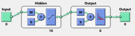
To set up the network architecture, we can use the patternnet function:
net is a model object that contains several modifiable properties that define the actions to be performed on the neural network.
A full description of neural network properties can be found here.
Assigning network training and hyperparameters
Aside from the number of nodes in the hidden layer, we can specify several training and hyperparameters.
First, I will set the train:test:validation split ratios: 7:2:1.
We can also modify the maximum number of epochs to run.
Because this is a binary classification problem, the default loss function is cross-entropy. To set the loss function manually, we can use the code below. Additional loss function arguments can be found here.
Training and Evaluating the Shallow Neural Network
Training the model
Now we can use the train function to train the neural network. It outputs the trained neural network object with additional properties and the record from training.
An interactive UI will also pop up during the training phase to show the model progress, which should look like the figure shown below.
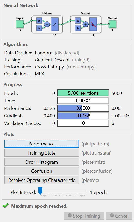
Another cool note about the default setting for the DLT is that it performs early stopping to avoid overfitting! So even if we specify a large number of epochs to train on, it will stop after the cost converges to a stable value.
Computing the prediction error
The trainedNet object also acts as a method to make predictions and takes in the input dataset as an argument. We can also evaluate the model performance using the perform function.
Visualizing and interpreting the model results
Cost curves
Now that we have a general sense of how the shallow neural network performed, we can visualize the results.
One diagnostic plot we can make is to visualize how the cost changes as a function of the number of epochs.
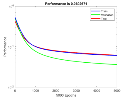
The cost computed from the training, validation, and test set seems to stabilize around 5,000 epochs.
The code to generate the cost curve is shown below.
Confusion matrix
To evaluate the model accuracy, we can plot a confusion matrix of our predictions showing average accuracy using the plotconfusion function.
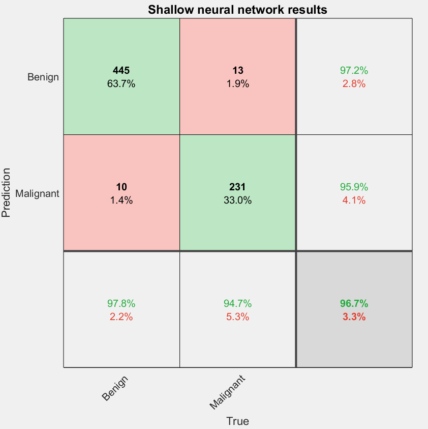
The diagonal cells are correct predictions while off-diagonal cells are incorrect predictions. The values in the far-right column are the precision while the bottom row contains the recall values. Overall, the model had an accuracy of 96.3%, which is not bad considering the number of nodes in the hidden layer was selected arbitrarily without optimization.
The code to generate the confusion matrix is shown below.
Receiver Operating Characteristic (ROC) Curves
Finally, if we want to get a sense of the precision and recall from the model, we can generate the ROC curves for the training, test, and validation sets. This was generated using the interactive UI.
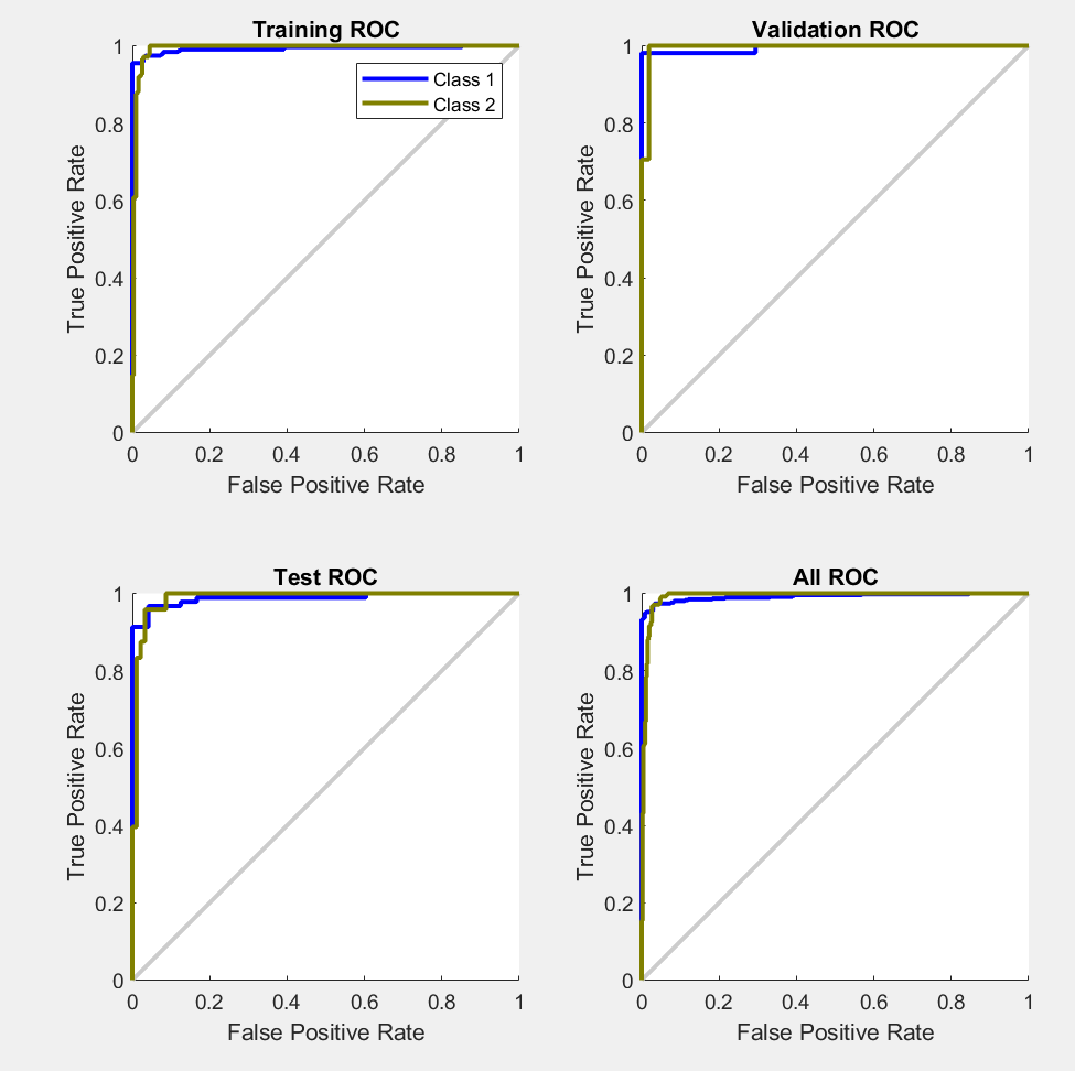
The ROC is close to 1, telling us that the model can distinguish between the two classes (benign/malignant).
Hyperparameter tuning with the Shallow Neural Network
Unfortunately, there is no built-in MATLAB function that performs hyperparameter tuning on neural networks to obtain an optimal model as of this writing.
The code block below performs a search to sample 2 through 20 nodes in the hidden layer using the DLT.
Let’s now visualize the errors.
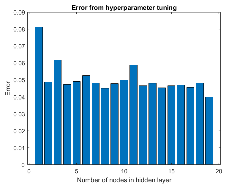
In our particular case, 20 nodes in the hidden layer minimizes the error value.
If we were interested in grabbing the optimal model for downstream analyses and finer tuning, we could grab the model in the models cell array.
The code used to generate the error bars.
Summary
This article provides a quick introduction to using some of the Deep Learning Toolbox (DLT) functionality and trains a Shallow Neural Network on a relatively simple dataset.
Additionally, we went over how to visualize the outputs from the model and briefly described how to interpret some of our results.
In the next article, we’ll implement deep neural network architectures using the DLT.
References
[Breast Cancer Wisconsin (Diagnostic) Data Set] W.N. Street, W.H. Wolberg, and O.L. Mangasarian. Nuclear feature extraction for breast tumor diagnosis. IS&T/SPIE 1993 International Symposium on Electronic Imaging: Science and Technology, volume 1905, pages 861–870, San Jose, CA, 1993. link